R Functions
Custom Figures
Download RFunctions1.R (GitHub)
-
dbplot() is a dot plot/box plot that displays individual data points, with automatic jittering when needed.
Its predecessor,
tplot(), was written over a decade ago. This newdbplot()builds upon it, offering enhanced functionality. Whilebeeswarm()in beeswarm package provides similar capabilities,dbplot()includes controls that better align with my taste and preferences.Inputs
Onlyyis absolutely required.Main arguments
yA numeric vector to be plotted.gA grouping vector.clustering_distanceControls which data points are considered part of the same cluster and thus jittered.- If
NULL, the function determines a reasonable value, and it is returned ifoutput=TRUE. - Setting
clustering_distance=0disables jittering.
- If
jitter_amountControls jitter distance.- If
NULL, the function determines a reasonable value, and it is returned ifoutput=TRUE. - Setting
jitter_amount=0disables jittering.
- If
outputIf TRUE, returns the clustering result,clustering_distance, andjitter_amount.group_namesA vector of group names, defaulting to the factor levels ofg.group_positionsBy default, data are plotted atx=1, 2, 3, ...unlessgroup_positionsare specified.
Color and Point Character
indiv_colA vector of individual colors fory.group_colSpecifies group colors,- Each group can have different colors, but this is redundant information.
- If a single color is provided, all data points are drawn in that color.
indiv_pchSeeindiv_col.group_pchSeegroup_col.
Handling Missing Group
NA_as_groupIf TRUE, missing values ingare treated as a separate group.NA_group_nameDefaults to "Missing".NA_group_positionThe plotting position of the missing group, defaulting to the far right.NA_group_colThe color for the "Missing" group.NA_group_pchThe pch (plotting character) for the "Missing" group.
Boxplot
box_colBoxplot colors, which can be specified for each group.NA_box_colBoxplot color for the "Missing" group.
Other Specifications
grid_xDraws vertical grid lines at specified values. (a little silly)grid_yDraws horizontal grid lines at specified values.show_nIf TRUE, displays sample sizes.xaxisIf FALSE, group names will not be shown.yaxisIf FALSE, y-axis will not be drawn.
Figure Type Options
fig_typeFigure type options.b: Boxplotd: Dot plotdb: Dot over boxplotbd: Box over dot plot (very silly)
NA_fig_typeFigure type for "Missing" group.
Additional Inputs
grid_parA list of parameters to pass to theabline() function for drawing grid lines. (col ,lty ,lwd ).
plot() ,points() ,boxplot() functions.plot()main ,sub ,xlab ,ylab ,xlim ,ylim ,axes ,frame.plot .points()cex ,bg .boxplot()range ,notch ,border ,boxwex .
Example
set.seed(620)
y <- rnorm(100, mean=100, sd=40)
g <- factor(sample(c('C','B','R'), length(y), rep=TRUE), levels=c('C','B','R'))
some_factor <- sample(c('A','B'), length(y), rep=TRUE)
    color_map <- c('A'='darkorange', 'B'='mediumslateblue')
    colors <- color_map[some_factor]
        y[ sample(seq_along(y), 5, rep=FALSE) ] <- NA
        g[ sample(seq_along(g), 4, rep=FALSE) ] <- NA

dbplot(y, g, group_names=c('Cat','Bat','Rat'),
           indiv_col=colors, group_pch=19,
           NA_as_group=TRUE, NA_group_name='?', NA_group_position=5,
           box_col=c('grey80','grey90','lightgoldenrodyellow'),
           grid_y=seq(0,250,by=50), show_n=TRUE,
           fig_type=c('b','d','db'), NA_fig_type='d',
           grid_par=list(col='skyblue', lty=1, lwd=1),
           clustering_distance=NULL, jitter_amount=NULL,
           ylim=c(0,250), xlab='Animal', ylab='Score', # passed to plot()
           cex=1.2, # passed to points()
           boxwex=0.6, border='royalblue' # passed to boxplot()
           )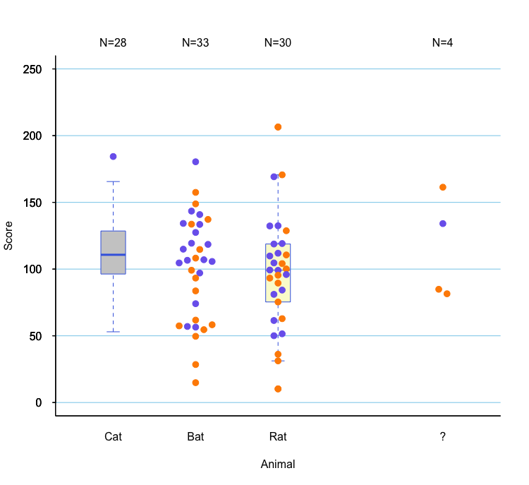
-
The kmplot() function generates Kaplan-Meier survival curves with various customization options, including a flexible "number at risk" table:
- The ability to customize the order of appearance to approximately match the curves.
- The ability to specify the time points where numbers are displayed.
Other functionalities are demonstrated in the example below.
Inputs
Main Arguments
kmOutput ofsurvfit()markTick mark style. The same aspch.simpleIf TRUE, the 'at risk' table will not be produced.xaxis.atSpecifies time positions where 'at risk' numbers are computed and displayed.xaxis.labLabels for the x-axis. Useful e.g., when time is in days but labels in year are preferred.
line Specifications
lty.survLine type for survival curveslwd.survLine width for survival curvescol.survColor for survival curveslty.ciLine type for confidence intervalslwd.ciLine width for confidence intervalscol.ciColor for confidence intervals
At Risk Table
group.namesNames displayed in the 'at risk' table and legend.group.orderReorders groups in the 'at risk' table to approximately match appearance of survival curves.extra.left.marginAdds extra space when group names are long.label.n.at.riskIf TRUE, labels the 'N at risk' table.draw.linesDraws lines to specifies survival curves. (Not sure why this is optional)cex.axisControls cex.axis and the text size of the 'N at risk' table.
Figure Appearances
xlabX-axis labelylabY-axis labelmainPlot titlexlmPassed to xlimylmPassed to ylim
Grid
gridIf TRUE, draws grid lines. Vertical lines appear atxaxis.atlocations, and horizontal lines atpretty(0,1)locations.lty.gridLine type for gridlwd.gridLine width for gridcol.gridColor for grid
Legend
legendEnables/disables the legendloc.legendControls legend position
Other
addIf TRUE, adds to an existing plot.returnOutputIf TRUE, returns the output ofsurvfit()....Additional arguments passed topar().
Example
require(survival)
kma <- survfit( Surv(time, status) ~ rx + adhere, data=colon )
kmplot(kma, mark='', simple=FALSE,
    xaxis.at=c(0, 0.5, 1:9)*365, xaxis.lab=c(0, 0.5, 1:9), # n.risk.at
    lty.surv=c(1,2), lwd.surv=1, col.surv=c(1,1,2,2,4,4), # survival.curves
    col.ci=0, # confidence intervals not plotted
    group.names=c('Obs ','Obs tumor adh','Lev','Lev tumor adh','Lev+5FU ','Lev+5FU tumor adh'), # Change group names
    group.order=c(5,3,1,6,4,2), # order of appearance in the n.risk.at table and legend.
    extra.left.margin=6, label.n.at.risk=FALSE, draw.lines=TRUE,
    cex.axis=0.8, xlab='Years', ylab='Survival Probability', # labels
    grid=TRUE, lty.grid=1, lwd.grid=1, col.grid='bisque',
    legend=TRUE, loc.legend='bottomleft',
    cex.lab=0.8, xaxs='r', bty='L', las=1, tcl=-0.2 # other parameters passed to plot()
)
title(main='Chemotherapy for stage B/C colon cancer', adj=.1, font.main=1, line=0.5, cex.main=1)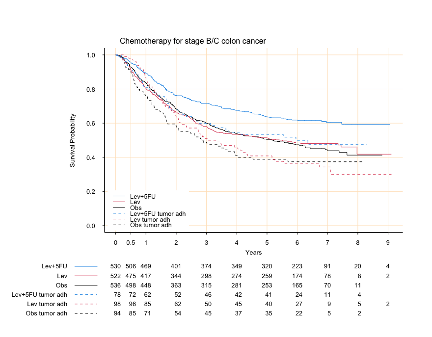
-
shadeDist draws a Normal curve or t-distribution curve and shade the specified region. I wrote this for teaching Biostats 1.
- Either one of
dfor "meanandsd" needs to be specified. - The shaded region is specified either by
LEFT,RIGHT, orBETWEEN. More than one of these can be used.
shadeDist(mean=120, sd=8, BETWEEN=c(116, 132), ylab='Density')
title(main='Normal(120, 8)', font.main=3, adj=0)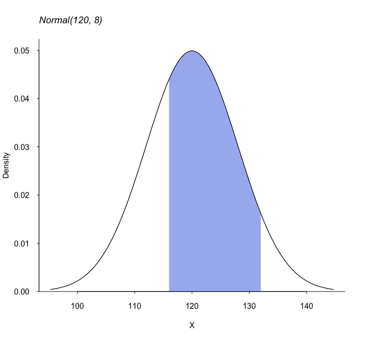
- Either one of
-
show.colors() shows all 657 named colors in R. You can select a color and display its name by running
colors()[n].Example
show.colors()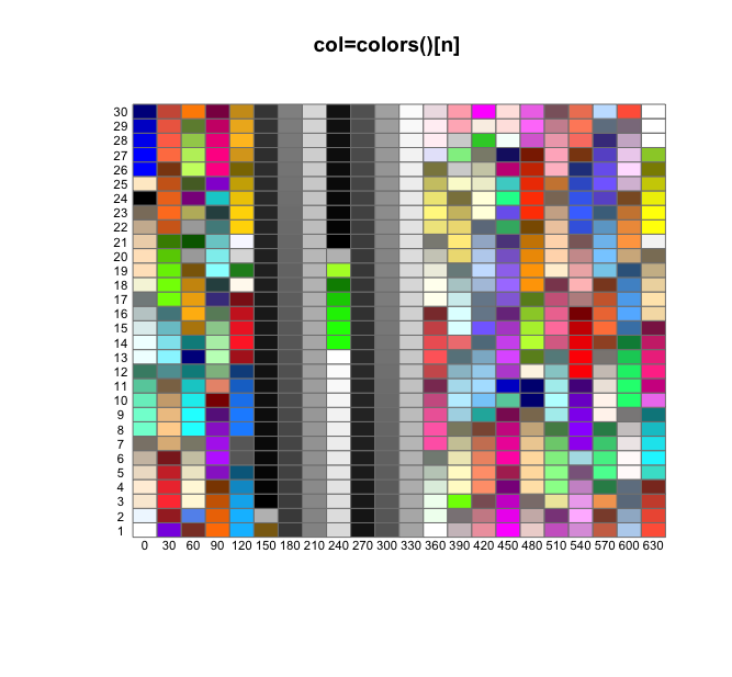
colors()[139] [1] "forestgreen" -
text.with.bg() adds text to a plot with a background rectangle.
Inputs
Main Arguments
x.posPosition of the text box on the x-axis (upper-left corner).y.posPosition of the text box on the y-axis (upper-left corner).txtThe text to be displayed.
Padding & Sizing
x.padHorizontal padding around the text, relative to the plot size (%).y.padVertical padding around the text, relative to the plot size (%).
Appearance
colColor of the text.bkgrBackground color of the text box. Set toNAfor transparency.borderColor of the rectangle border. Defaults toNA(no border).
Additional Arguments
...Passed to `text()` and `strwidth()`/`strheight()`, allowing customization of font size (`cex`) and style (`font`),
Example
set.seed(620)
x <- sample(4:14, 100, replace=TRUE) + rnorm(100,0,1)
y <- x + rnorm(100, 0, 3)
x[100] <- 15.2 ; y[100] <- 3.1

plot(x,y, xlim=c(0,20), ylim=c(0,20), panel.first=grid(nx=NULL, ny=NULL,lty=1, col='lightblue'))

txt <- paste('Say something','\n','interesting here.', sep='')
text.with.bg(x.pos=15.5, y.pos=2.5, txt=txt, col='royalblue', bkgr='thistle1', x.pad=2, y.pad=2,
              border='dodgerblue', cex=0.8, font=4, family='serif')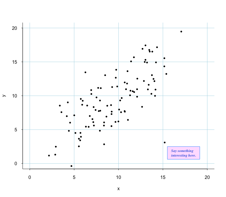
-
Deprecated.
tplot()is no longer maintained. Please usedbplot()instead.tplot() is an alternative to boxplot(). It allows individual data points to be displayed, either in the foreground or background, with jittering if necessary.
Example
This example demonstrates the various options available in tplot(). While this particular example is not the most effective way to visualize these data -due to unnecessary variation in color and point type- it highlights the function's customization features.colandpchcan be specified at either the individual or group level. In this example,colis set at the individual level, whilepchis assigned at the group level, though this pch variation is unnecessary.- The
typeargument controls the plot style: b (box only), d (dots only), bd (box in front of dots), and db (dots in front of the box). - Points that are closer than
distare jittered bydist. This implementation may be incorrect. -try different values to see its impact. - Box colors and borders are controlled by the
boxcolandboxborderarguments. - The
boxplot.parsargument is passed directly toboxplot(), allowing further customization.
Example
set.seed(100)
y <- rnorm(80, 26, 9)
sex <- factor(sample(c('Female', 'Male'), 80, TRUE))
group <- paste('Group ', sample(1:4, 40, prob = c(2,5,4,1), replace = TRUE), sep='')

d <- data.frame(y, sex, group)
        rm(y,sex,group)

tplot(y ~ group, data=d, ylim=c(0,50),
    las=1, cex=1, cex.axis=1, bty='L',
    show.n=TRUE, dist=0.5, jit=0.07, type=c('b','bd','db','d'),
    group.pch=TRUE, pch=c(15,17,20,19),
    group.col=FALSE, col=c('orange','darkgreen')[c(sex)],
    boxcol=c('dodgerblue','magenta', 'lightgrey', 'pink'),
    boxborder=grey(0.2),
    boxplot.pars=list(notch=TRUE, boxwex=0.5)
)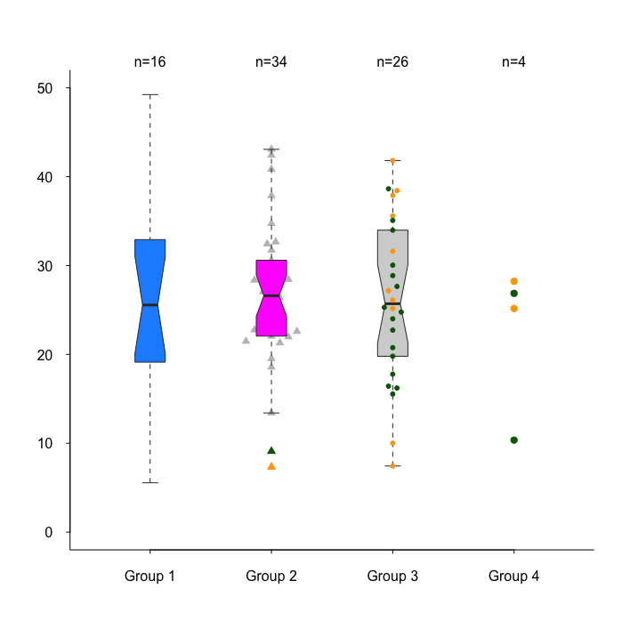
-
Deprecated.
jmplot()plots the joint distribution along with marginal distributions on each margin. The parametersdist(which controls jitter) andjit(which sets the jitter amount) are currently swapped for unknown reasons. I'll fix it someday. In the meantime, ggplot2 has this covered.Example
set.seed(1220)

x <- rexp(100)
y <- rexp(100)
levels <- as.factor(sample(c("Male","Female"), 100, TRUE))
co <- c('brown','royalblue')[as.numeric(levels)]

jmplot(x, y, levels, col=co, pch=19, main='Title', show.n=TRUE)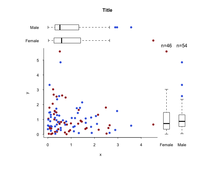
-
Deprecated. (Discrete scatter plot) The idea was to show continuous data with lots of ties effectively. This is no longer being developed. Use jitter() function carefully.